Stochastic Gradient Descent with Restarts

Simply finding a learning rate to undergo gradient descent will help minimize the loss of a neural network. However, there are additional methods that can make this process smoother, faster, and more accurate.

The first technique is Stochastic Gradient Descent with Restarts (SGDR), a variant of learning rate annealing, which gradually decreases the learning rate through training.

Each step decreases in size

There are different methods of annealing, different ways of decreasing the step size. One popular way is to decrease learning rates by steps: to simply use one learning rate for the first few iterations, then drop to another learning rate for the next few iterations, then drop the learning rate further for the next few iterations. Another variant would be to linearly decrease the learning rate with each iteration.

Decreasing learning rate by steps

Linearly decrease learning rate

SGDR uses cosine annealing, which decreases learning rate in the form of half a cosine curve, like so:

This is a good method because we can start out with relatively high learning rates for several iterations in the beginning to quickly approach a local minimum, then gradually decrease the learning rate as we get closer to the minimum, ending with several small learning rate iterations.

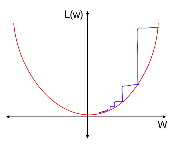
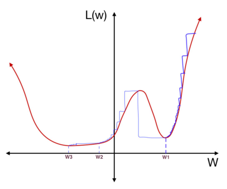
However, we may find ourselves in a local minimum where a small change in weights would result in a large change in loss. In this loss function below, through training, we’ve landed in a local minimum.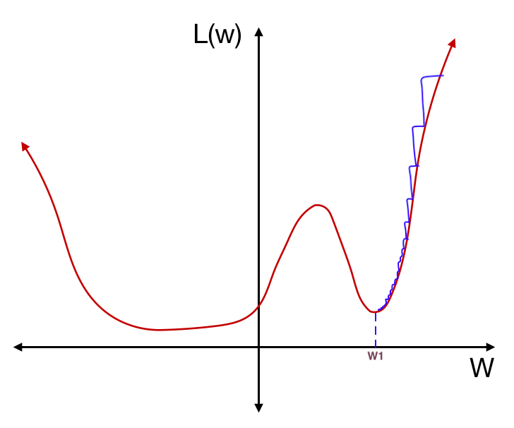 

If we test this network on a different dataset, however, the loss function might be slightly different. A small shift of the loss function in this local minimum will result in a large change of loss:

Suddenly, this local minimum is a terrible solution. On the other hand, if we had found a solution in this flatter trough:

even if a different dataset shifts the loss function a little, the loss would stay relatively stable:

This flatter trough is better as it offers both an accurate and stable solution. It is more generalized; that is, it has a higher ability to react to new data. In order to find a more stable local minimum, we can increase the learning rate from time to time, encouraging the model to “jump” from one local minimum to another if it is in a steep trough. This is the “restarts” in SGDR.

Increasing the learning rates every few iterations to “restart” the gradient descent

In the first “half cosine” period in the graph above, we descend into a local minimum, like so:

Suddenly, we increase the learning rate, taking a big step in the next iteration:

 

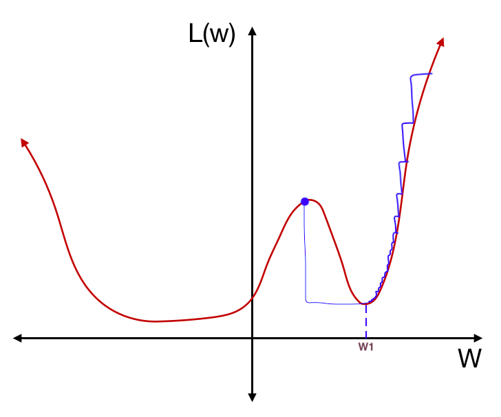
In the second “half cosine” period, we descend into another local minimum.

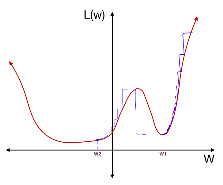
And then we sharply increase the learning rate again. Only this time, because we are in a more stable region of the loss function, this “restart” does not take us out of the local minimum:

Finally, we gradually decrease the learning rate again until we minimize the loss function, finding a stable solution.

Each of these ‘periods’ is known as a cycle, and in training our neural network, we can choose the number of cycles and the length of each cycle ourselves. Also, since we are gradually decreasing the learning rate, it is better to start with a learning rate slightly larger than the optimum learning rate (how do you determine the optimum learning rate? Click here). It is also important to choose a learning rate large enough to allow the function to jump to a different minimum when “reset”.

You can also increase the cycle length after each cycle, like so:

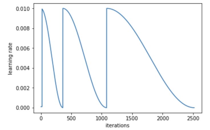
This seems to output a better, more accurate result as it allows us to find the minimum point in a stable region more precisely.